44 how to display data labels in excel
Custom Chart Data Labels In Excel With Formulas - How To Excel At Excel Follow the steps below to create the custom data labels. Select the chart label you want to change. In the formula-bar hit = (equals), select the cell reference containing your chart label's data. In this case, the first label is in cell E2. Finally, repeat for all your chart laebls. DataLabels.ShowValue property (Excel) | Microsoft Docs This example enables the value to be shown for the data labels of the first series, on the first chart. This example assumes that a chart exists on the active worksheet. VB. Copy. Sub UseValue () ActiveSheet.ChartObjects (1).Activate ActiveChart.SeriesCollection (1) _ .DataLabels.ShowValue = True End Sub.
How to add multiple data labels in excel Batch add all data labels from different column in an Excel chart. 1. Right click the data series in the chart, and select Add Data Labels > Add Data Labels from the context menu to add data labels. 2. Right click the data series, and select …Adding data labels is dependent on MS Excel version.

How to display data labels in excel
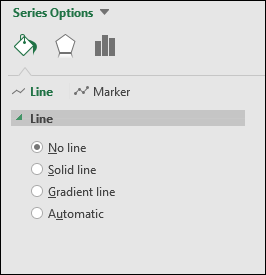
Display data point labels outside a pie chart in a paginated report ... To display data point labels inside a pie chart. Add a pie chart to your report. For more information, see Add a Chart to a Report (Report Builder and SSRS). On the design surface, right-click on the chart and select Show Data Labels. To display data point labels outside a pie chart. Create a pie chart and display the data labels. Open the ... › documents › excelHow to display text labels in the X-axis of scatter chart in ... Select the data you use, and click Insert > Insert Line & Area Chart > Line with Markers to select a line chart. See screenshot: 2. Then right click on the line in the chart to select Format Data Series from the context menu. See screenshot: 3. In the Format Data Series pane, under Fill & Line tab, click Line to display the Line section, then ... support.microsoft.com › en-us › officeEdit titles or data labels in a chart - support.microsoft.com To reposition all data labels for an entire data series, click a data label once to select the data series. To reposition a specific data label, click that data label twice to select it. This displays the Chart Tools , adding the Design , Layout , and Format tabs.
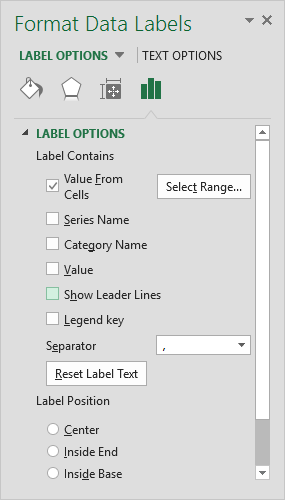
How to display data labels in excel. Trendline.DataLabel property (Excel) | Microsoft Docs In this article. Returns a DataLabel object that represents the data label associated with the trendline. Read-only. Syntax. expression.DataLabel. expression A variable that represents a Trendline object.. Remarks. To turn on data labels for a trendline, you need to set the DisplayEquation property or the DisplayRSquared property to True.. Support and feedback support.microsoft.com › en-us › officeAdd or remove data labels in a chart - support.microsoft.com Right-click the data series or data label to display more data for, and then click Format Data Labels. Click Label Options and under Label Contains , select the Values From Cells checkbox. When the Data Label Range dialog box appears, go back to the spreadsheet and select the range for which you want the cell values to display as data labels. › format-data-labels-in-excelFormat Data Labels in Excel- Instructions - TeachUcomp, Inc. Nov 14, 2019 · Then select the “Format Data Labels…” command from the pop-up menu that appears to format data labels in Excel. Using either method then displays the “Format Data Labels” task pane at the right side of the screen. Format Data Labels in Excel- Instructions: A picture of the “Format Data Labels” task pane in Excel. What Are Data Labels in Excel (Uses & Modifications) - ExcelDemy Removing Data Labels from an Excel Chart: To erase data labels from an Excel chart, please follow the steps below. Steps: Simply click on the chart that you would like to remove the data labels from. It shows the Chart Tools, including the Design and also Format tabs.
How To Add Data Labels In Excel ~ Pvkngcchittoor Now we need to add the flavor names to the label.now right click on the label and click format data labels. To add or move data labels in a chart, you can do as below steps: Source: . Data labels are used to display source data in a chart directly. Change position of data labels. Source: . The column chart will appear. › documents › excelHow to add data labels from different column in an Excel chart? This method will introduce a solution to add all data labels from a different column in an Excel chart at the same time. Please do as follows: 1. Right click the data series in the chart, and select Add Data Labels > Add Data Labels from the context menu to add data labels. 2. How to Add Labels to Scatterplot Points in Excel - Statology Step 3: Add Labels to Points. Next, click anywhere on the chart until a green plus (+) sign appears in the top right corner. Then click Data Labels, then click More Options…. In the Format Data Labels window that appears on the right of the screen, uncheck the box next to Y Value and check the box next to Value From Cells. How do you label data points in Excel? - profitclaims.com Please do as follows: 1. Right click the data series in the chart, and select Add Data Labels > Add Data Labels from the context menu to add data labels. 2. Right click the data series, and select Format Data Labels from the context menu. 3.
Data Labels in Excel Pivot Chart (Detailed Analysis) Add a Pivot Chart from the PivotTable Analyze tab. Then press on the Plus right next to the Chart. Next open Format Data Labels by pressing the More options in the Data Labels. Then on the side panel, click on the Value From Cells. Next, in the dialog box, Select D5:D11, and click OK. How to Show Pie Chart Data Labels in Percentage in Excel - ExcelDemy While using an Excel Pie Chart, showing the percentage in data labels helps us to understand the difference between the sectors at a glance, also it can give a better look of the chart. So in this article, I'll show 3 useful methods to show the percentage in the data labels of the Excel Pie Chart with clear steps and vivid illustrations. How to add text labels on Excel scatter chart axis - Data Cornering Add dummy series to the scatter plot and add data labels. 4. Select recently added labels and press Ctrl + 1 to edit them. Add custom data labels from the column "X axis labels". Use "Values from Cells" like in this other post and remove values related to the actual dummy series. Change the label position below data points. How to add data labels in excel to graph or chart (Step-by-Step) Add data labels to a chart. 1. Select a data series or a graph. After picking the series, click the data point you want to label. 2. Click Add Chart Element Chart Elements button > Data Labels in the upper right corner, close to the chart. 3. Click the arrow and select an option to modify the location. 4.
30 What Is A Data Label In Excel - Labels Database 2020
How to Mail Merge Labels from Excel to Word (With Easy Steps) - ExcelDemy Download Practice Workbook. Step by Step Procedures to Mail Merge Labels from Excel to Word. STEP 1: Prepare Excel File for Mail Merge. STEP 2: Insert Mail Merge Document in Word. STEP 3: Link Word and Excel for Merging Mail Labels. STEP 4: Select Recipients. STEP 5: Edit Address Labels.

How to Create a Geographical Map Chart in Microsoft Excel
How to Create and Customize a Treemap Chart in Microsoft Excel Simply click that text box and enter a new name. Next, you can select a style, color scheme, or different layout for the treemap. Select the chart and go to the Chart Design tab that displays. Use the variety of tools in the ribbon to customize your treemap. For fill and line styles and colors, effects like shadow and 3-D, or exact size and ...

How to sort in Excel Tables
chandoo.org › wp › change-data-labels-in-chartsHow to Change Excel Chart Data Labels to Custom Values? May 05, 2010 · Now, click on any data label. This will select “all” data labels. Now click once again. At this point excel will select only one data label. Go to Formula bar, press = and point to the cell where the data label for that chart data point is defined. Repeat the process for all other data labels, one after another. See the screencast.

Excel 2013 Tutorial Formatting Data Labels Microsoft Training Lesson 28.6 - YouTube
How to Display Percentage in an Excel Graph (3 Methods) Display Percentage in Graph. Select the Helper columns and click on the plus icon. Then go to the More Options via the right arrow beside the Data Labels. Select Chart on the Format Data Labels dialog box. Uncheck the Value option. Check the Value From Cells option.

How To Use Dynamic Data Labels To Create Interactive Excel Charts
excel - How to not display labels in pie chart that are 0% - Stack Overflow Generate a new column with the following formula: =IF (B2=0,"",A2) Then right click on the labels and choose "Format Data Labels". Check "Value From Cells", choosing the column with the formula and percentage of the Label Options. Under Label Options -> Number -> Category, choose "Custom". Under Format Code, enter the following:

30 How To Add Label To Excel Chart - Labels Database 2020
How to Convert Excel to Word Labels (With Easy Steps) Step by Step Guideline to Convert Excel to Word Labels Step 1: Prepare Excel File Containing Labels Data. First, list the data that you want to include in the mailing labels in an Excel sheet.For example, I want to include First Name, Last Name, Street Address, City, State, and Postal Code in the mailing labels.; If I list the above data in excel, the file will look like the below screenshot.
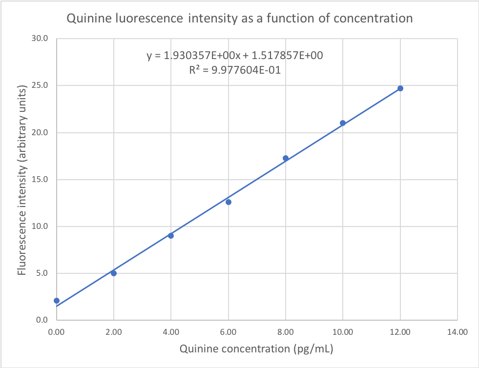
Statistics in Analytical Chemistry - Excel™
How to Print Labels from Excel - Lifewire Select Mailings > Write & Insert Fields > Update Labels . Once you have the Excel spreadsheet and the Word document set up, you can merge the information and print your labels. Click Finish & Merge in the Finish group on the Mailings tab. Click Edit Individual Documents to preview how your printed labels will appear. Select All > OK .
Custom Chart Labels Using Excel 2013 | MyExcelOnline
› charts › dynamic-chart-dataCreate Dynamic Chart Data Labels with Slicers - Excel Campus Feb 10, 2016 · Typically a chart will display data labels based on the underlying source data for the chart. In Excel 2013 a new feature called “Value from Cells” was introduced. This feature allows us to specify the a range that we want to use for the labels. Since our data labels will change between a currency ($) and percentage (%) formats, we need a ...
How To Use Dynamic Data Labels To Create Interactive Excel Charts
How to Add Two Data Labels in Excel Chart (with Easy Steps) Step 4: Format Data Labels to Show Two Data Labels. Here, I will discuss a remarkable feature of Excel charts. You can easily show two parameters in the data label. For instance, you can show the number of units as well as categories in the data label. To do so, Select the data labels. Then right-click your mouse to bring the menu.

Creating Pie Chart and Adding/Formatting Data Labels (Excel) - YouTube
support.microsoft.com › en-us › officeEdit titles or data labels in a chart - support.microsoft.com To reposition all data labels for an entire data series, click a data label once to select the data series. To reposition a specific data label, click that data label twice to select it. This displays the Chart Tools , adding the Design , Layout , and Format tabs.

Format Data Labels in Excel- Instructions | Microsoft excel, Microsoft, Bar chart
› documents › excelHow to display text labels in the X-axis of scatter chart in ... Select the data you use, and click Insert > Insert Line & Area Chart > Line with Markers to select a line chart. See screenshot: 2. Then right click on the line in the chart to select Format Data Series from the context menu. See screenshot: 3. In the Format Data Series pane, under Fill & Line tab, click Line to display the Line section, then ...

30 What Is Data Label In Excel - Labels Design Ideas 2020
Display data point labels outside a pie chart in a paginated report ... To display data point labels inside a pie chart. Add a pie chart to your report. For more information, see Add a Chart to a Report (Report Builder and SSRS). On the design surface, right-click on the chart and select Show Data Labels. To display data point labels outside a pie chart. Create a pie chart and display the data labels. Open the ...

How to create an Excel map chart
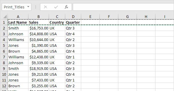
Print Titles in Excel - Easy Excel Tutorial

Format Data Labels in Excel- Instructions - TeachUcomp, Inc.
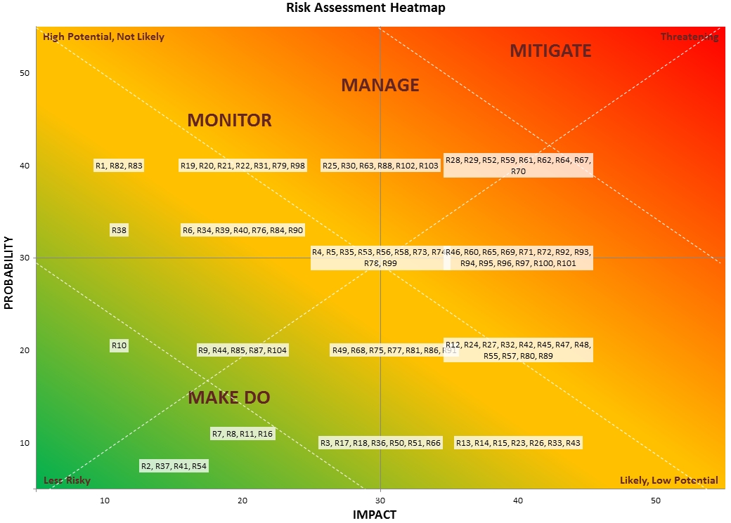
How to Create a Risk Heatmap in Excel - Part 2 - Risk Management Guru
How to Make an XY Graph on Excel | Techwalla.com
Post a Comment for "44 how to display data labels in excel"