40 how to change data labels in excel 2013

formatting - How to format Microsoft Excel data labels without trailing ... One way to do this, is like so: If your numbers are in column B, apply this formula for column C =B1=INT (B1) This will show TRUE if the data is of INT data type (no decimal precision) and FALSE if not. How to Create a Timeline Chart in Excel - Automate Excel This tutorial will demonstrate how to create a timeline chart in all versions of Excel: 2007, 2010, 2013, 2016, and 2019. Timeline Chart ... Change the chart type of the newly-created data series. ... right-click on any of the data labels and open the Format Data Labels task pane.

How to Add Data Tables to Charts in Excel 2013 - dummies To add a data table to your selected chart and position and format it, click the Chart Elements button next to the chart and then select the Data Table check box before you select one of the following options on its continuation menu: With Legend Keys to have Excel draw the table at the bottom of the chart, including the color keys used in the ...

How to change data labels in excel 2013

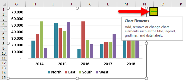
How to Show Percentage Change in Excel Graph (2 Ways) 31.5.2022 · This article will illustrate how to show the percentage change in an Excel graph. Using an Excel graph can present you the relation between the data in an eye-catching way. Showing partial numbers as percentages is easy to understand while analyzing data. In the following dataset, we have a company’s Profit during the period March to September. Change axis labels in a chart - support.microsoft.com Right-click the category labels you want to change, and click Select Data. In the Horizontal (Category) Axis Labels box, click Edit. In the Axis label range box, enter the labels you want to use, separated by commas. For example, type Quarter 1,Quarter 2,Quarter 3,Quarter 4. Change the format of text and numbers in labels How to add or move data labels in Excel chart? - ExtendOffice To add or move data labels in a chart, you can do as below steps: In Excel 2013 or 2016. 1. Click the chart to show the Chart Elements button .. 2. Then click the Chart Elements, and check Data Labels, then you can click the arrow to choose an option about the data labels in the sub menu.See screenshot:

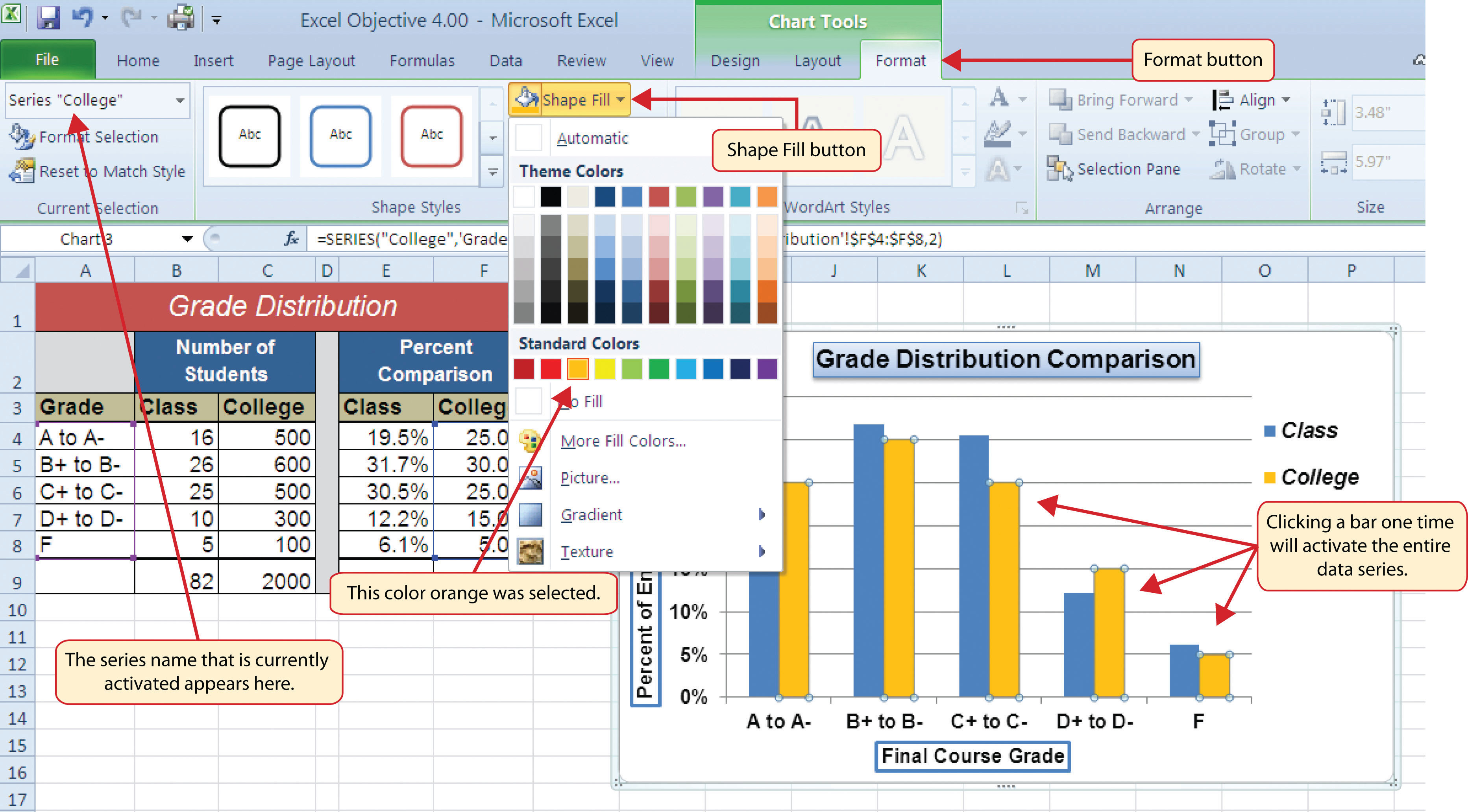
How to change data labels in excel 2013. Custom Chart Data Labels In Excel With Formulas - How To Excel At Excel Select the chart label you want to change. In the formula-bar hit = (equals), select the cell reference containing your chart label's data. In this case, the first label is in cell E2. Finally, repeat for all your chart laebls. If you are looking for a way to add custom data labels on your Excel chart, then this blog post is perfect for you. Format Data Labels in Excel- Instructions - TeachUcomp, Inc. To do this, click the "Format" tab within the "Chart Tools" contextual tab in the Ribbon. Then select the data labels to format from the "Chart Elements" drop-down in the "Current Selection" button group. Then click the "Format Selection" button that appears below the drop-down menu in the same area. How to change chart axis labels' font color and size in Excel? Apply conditional formatting to fill columns in a chart. By default, all data point in one data series are filled with same color. Here, with the Color Chart by Value tool of Kutools for Excel, you can easily apply conditional formatting to a chart, and fill data points with different colors based on point values. Full Feature Free Trial 30-day! VBA to change data label in a chart - Compatibility btw Excel 2013 and ... It seems that Excel 2010 and 2013 work differently regarding to number format code in Macros. Due my limited access to Excel 2010, the solution was to duplicate the charts, change the labels as necessary and then switch the macro to show only the charts with the millions/thousands labels.

How to Add Data Labels in Excel - Excelchat | Excelchat In Excel 2013 And Later Versions In Excel 2013 and the later versions we need to do the followings; Click anywhere in the chart area to display the Chart Elements button Figure 5. Chart Elements Button Click the Chart Elements button > Select the Data Labels, then click the Arrow to choose the data labels position. Figure 6. Microsoft Excel 2010 vs 2013 vs 2016 vs 2019: Complete Guide This tool allows you to import higher levels of data. It comes with its language, Data Analysis Expression. Microsoft Excel 2013. New Look. Microsoft Excel 2016 flaunts a new and better look than what you are used to from the older versions. A start-up screen comes up when you launch it unlike the blank workbook from older versions. Edit titles or data labels in a chart Change the position of data labels. You can change the position of a single data label by dragging it. You can also place data labels in a standard position relative to their data markers. Depending on the chart type, you can choose from a variety of positioning options. On a chart, do one of the following: How to Make a Pie Chart in Excel & Add Rich Data Labels to The … 8.9.2022 · A pie chart is used to showcase parts of a whole or the proportions of a whole. There should be about five pieces in a pie chart if there are too many slices, then it’s best to use another type of chart or a pie of pie chart in order to showcase the data better. In this article, we are going to see a detailed description of how to make a pie chart in excel.

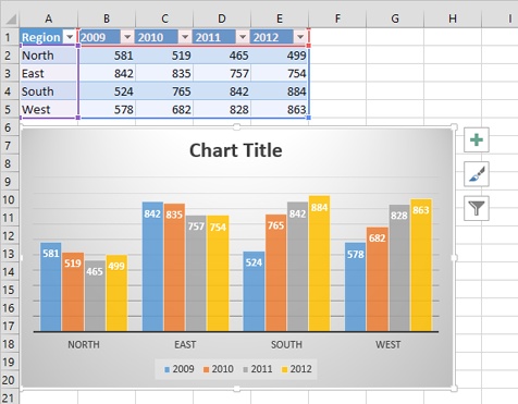
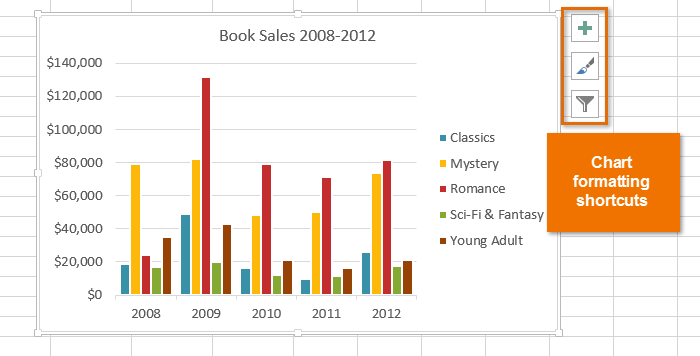
How to Change Excel Chart Data Labels to Custom Values? 5.5.2010 · Now, click on any data label. This will select “all” data labels. Now click once again. At this point excel will select only one data label. Go to Formula bar, press = and point to the cell where the data label for that chart data point is defined. Repeat the process for all other data labels, one after another. See the screencast. How to make a bar graph in Excel - Ablebits.com To create a cylinder, cone or pyramid graph in Excel 2016 and 2013, make a 3-D bar chart of your preferred type (clustered, stacked or 100% stacked) in the usual way, and then change the shape type in the following way: Select all the bars in your chart, right click them, and choose Format Data Series... from the context menu. support.microsoft.com › en-us › officeEdit titles or data labels in a chart - support.microsoft.com Change the position of data labels. You can change the position of a single data label by dragging it. You can also place data labels in a standard position relative to their data markers. Depending on the chart type, you can choose from a variety of positioning options. On a chart, do one of the following: Excel charts: add title, customize chart axis, legend and data labels Click anywhere within your Excel chart, then click the Chart Elements button and check the Axis Titles box. If you want to display the title only for one axis, either horizontal or vertical, click the arrow next to Axis Titles and clear one of the boxes: Click the axis title box on the chart, and type the text.

Adding rich data labels to charts in Excel 2013 | Microsoft ...

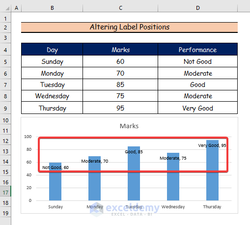
Move data labels - support.microsoft.com Click any data label once to select all of them, or double-click a specific data label you want to move. Right-click the selection > Chart Elements > Data Labels arrow, and select the placement option you want. Different options are available for different chart types.

Change the format of data labels in a chart

chandoo.org › wp › change-data-labels-in-chartsHow to Change Excel Chart Data Labels to Custom Values? May 05, 2010 · Now, click on any data label. This will select “all” data labels. Now click once again. At this point excel will select only one data label. Go to Formula bar, press = and point to the cell where the data label for that chart data point is defined. Repeat the process for all other data labels, one after another. See the screencast.

Excel 2013 Tutorial Formatting Data Labels Microsoft Training Lesson 28.6

support.microsoft.com › en-us › officeChange the format of data labels in a chart To get there, after adding your data labels, select the data label to format, and then click Chart Elements > Data Labels > More Options. To go to the appropriate area, click one of the four icons ( Fill & Line , Effects , Size & Properties ( Layout & Properties in Outlook or Word), or Label Options ) shown here.

How to add or move data labels in Excel chart?

Custom Data Labels with Colors and Symbols in Excel Charts - [How To ... Step 4: Select the data in column C and hit Ctrl+1 to invoke format cell dialogue box. From left click custom and have your cursor in the type field and follow these steps: Press and Hold ALT key on the keyboard and on the Numpad hit 3 and 0 keys. Let go the ALT key and you will see that upward arrow is inserted.

How to add or move data labels in Excel chart?

Change the format of data labels in a chart You can use leader lines to connect the labels, change the shape of the label, and resize a data label. And they’re all done in the Format Data Labels task pane. To get there, after adding your data labels, select the data label to format, and then click Chart Elements > …

Creating Pie Chart and Adding/Formatting Data Labels (Excel)

Changing Axis Labels in PowerPoint 2013 for Windows - Indezine Changing Horizontal (Category) Axis Labels . Now, let us learn how to change category axis labels. First select your chart. Then, click the Edit Data button as shown highlighted in red within Figure 7,below, within the Charts Tools Design tab of the Ribbon. This opens an instance of Excel with your chart data.

Excel charts: add title, customize chart axis, legend and ...

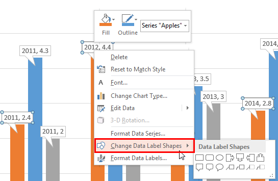
How to Customize Chart Elements in Excel 2013 - dummies To add data labels to your selected chart and position them, click the Chart Elements button next to the chart and then select the Data Labels check box before you select one of the following options on its continuation menu: Center to position the data labels in the middle of each data point

Change the format of data labels in a chart

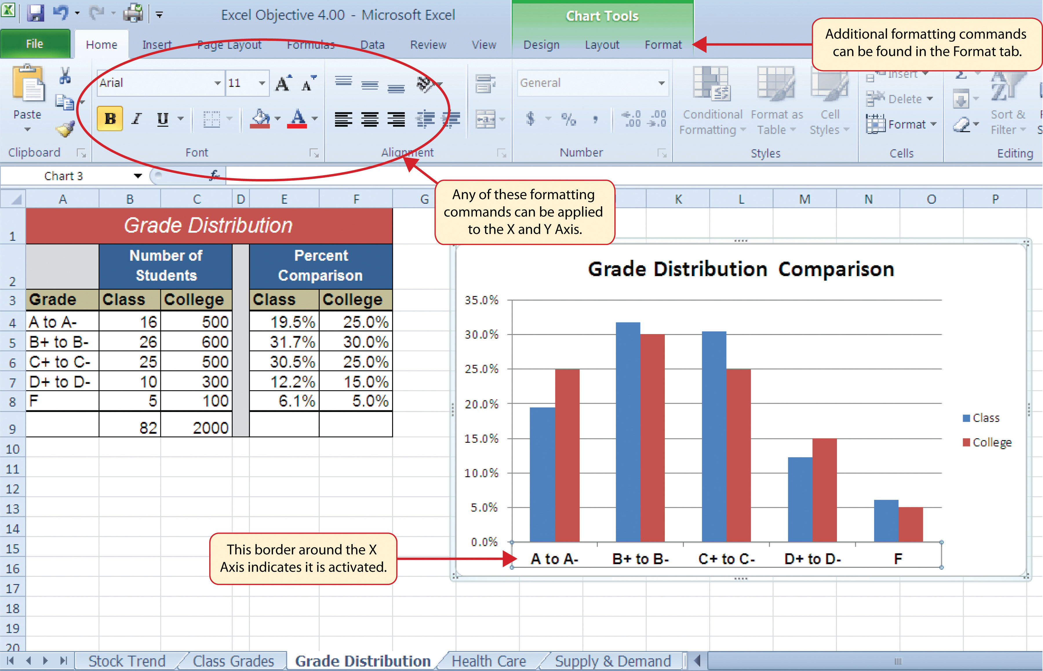
› documents › excelHow to change chart axis labels' font color and size in Excel? We can easily change all labels' font color and font size in X axis or Y axis in a chart. Just click to select the axis you will change all labels' font color and size in the chart, and then type a font size into the Font Size box, click the Font color button and specify a font color from the drop down list in the Font group on the Home tab.

How to Add Total Data Labels to the Excel Stacked Bar Chart ...

Add or remove data labels in a chart - support.microsoft.com Click Label Options and under Label Contains, pick the options you want. Use cell values as data labels You can use cell values as data labels for your chart. Right-click the data series or data label to display more data for, and then click Format Data Labels. Click Label Options and under Label Contains, select the Values From Cells checkbox.

Creating a simple competition chart - Microsoft Excel 2013

Custom data labels in a chart - Get Digital Help Press with mouse on "Add Data Labels". Press with mouse on Add Data Labels". Double press with left mouse button on any data label to expand the "Format Data Series" pane. Enable checkbox "Value from cells". A small dialog box prompts for a cell range containing the values you want to use a s data labels.

Formatting Charts

How to Make Charts and Graphs in Excel | Smartsheet 22.1.2018 · Step 1: Enter Data into a Worksheet. Open Excel and select New Workbook. Enter the data you want to use to create a graph or chart. In this example, we’re comparing the profit of five different products from 2013 to 2017. Be sure to include labels for your columns and rows. Doing so enables you to translate the data into a chart or graph with ...

Change the format of data labels in a chart

How to Create a Pareto Chart in Excel - Automate Excel To do that, right-click on any of the blue columns representing Series "Items Returned" and click "Format Data Series." Then, follow a few simple steps: Navigate to the Series Options tab. Change "Gap Width" to "3%." Step #7: Add data labels. It's time to add data labels for both the data series (Right-click > Add Data Labels).

Change the format of data labels in a chart

How to rotate axis labels in chart in Excel? - ExtendOffice Go to the chart and right click its axis labels you will rotate, and select the Format Axis from the context menu. 2. In the Format Axis pane in the right, click the Size & Properties button, click the Text direction box, and specify one direction from the drop down list. See screen shot below: The Best Office Productivity Tools

Custom Excel Chart Label Positions • My Online Training Hub

› excel › how-to-add-total-dataHow to Add Total Data Labels to the Excel Stacked Bar Chart Apr 03, 2013 · Step 4: Right click your new line chart and select “Add Data Labels” Step 5: Right click your new data labels and format them so that their label position is “Above”; also make the labels bold and increase the font size. Step 6: Right click the line, select “Format Data Series”; in the Line Color menu, select “No line”

How to change chart axis labels' font color and size in Excel?

How to Add Total Data Labels to the Excel Stacked Bar Chart 3.4.2013 · For stacked bar charts, Excel 2010 allows you to add data labels only to the individual components of the stacked bar chart. The basic chart function does not allow you to add a total data label that accounts for the sum of the individual components. Fortunately, creating these labels manually is a fairly simply process.

How To Show Or Hide Data Labels On MS Excel? | My Windows Hub

› show-percentage-change-in-excelHow to Show Percentage Change in Excel Graph (2 Ways) - ExcelDemy May 31, 2022 · This article will illustrate how to show the percentage change in an Excel graph. Using an Excel graph can present you the relation between the data in an eye-catching way. Showing partial numbers as percentages is easy to understand while analyzing data. In the following dataset, we have a company’s Profit during the period March to September.

Apply Custom Data Labels to Charted Points - Peltier Tech

Is there a way to change the order of Data Labels? Answer Rena Yu MSFT Microsoft Agent | Moderator Replied on April 4, 2018 Hi Keith, I got your meaning. Please try to double click the the part of the label value, and choose the one you want to show to change the order. Thanks, Rena ----------------------- * Beware of scammers posting fake support numbers here.

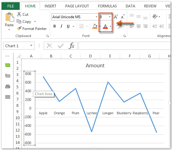
Change Callout Shapes for Data Labels in PowerPoint 2013 for ...

How to Create Mailing Labels in Word from an Excel List Note: If your label outlines aren't showing, go to Design > Borders, and select "View Gridlines." Step Three: Connect your Worksheet to Word's Labels. Before you can transfer the data from Excel to your labels in Word, you must connect the two. Back in the "Mailings" tab in the Word document, select the "Select Recipients" option.

Legends in Excel | How to Add legends in Excel Chart?

› how-to-create-excel-pie-chartsHow to Make a Pie Chart in Excel & Add Rich Data Labels to ... Sep 08, 2022 · How to Make Two Pie Charts with One Legend in Excel; Excel Pie Chart Labels on Slices: Add, Show & Modify Factors; How to Change Pie Chart Colors in Excel (4 Easy Ways) Add Labels with Lines in an Excel Pie Chart (with Easy Steps) How to Edit Pie Chart in Excel (All Possible Modifications) Create A Doughnut, Bubble and Pie of Pie Chart in Excel

Analyzing Data with Tables and Charts in Microsoft Excel 2013 ...

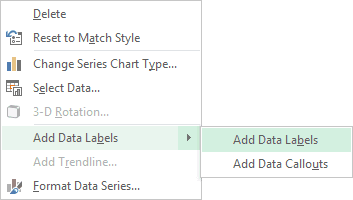
Adding rich data labels to charts in Excel 2013 | Microsoft 365 Blog To add a data label in a shape, select the data point of interest, then right-click it to pull up the context menu. Click Add Data Label, then click Add Data Callout . The result is that your data label will appear in a graphical callout. In this case, the category Thr for the particular data label is automatically added to the callout too.

Adding rich data labels to charts in Excel 2013 | Microsoft ...

How to Print Labels from Excel - Lifewire Choose Start Mail Merge > Labels . Choose the brand in the Label Vendors box and then choose the product number, which is listed on the label package. You can also select New Label if you want to enter custom label dimensions. Click OK when you are ready to proceed. Connect the Worksheet to the Labels

Add or remove data labels in a chart

How to change interval between labels in Excel 2013? I found the solution easily on the web. Just click on the axis on the chart -> then click on Format axis to the right -> Axis options -> Labels -> Under Interval between labels I should be able to specify interval units. In my case. There is No Interval Between Labels, it is missing. The only thing there is Label Position.

Custom Excel Chart Label Positions • My Online Training Hub

How to add data labels from different column in an Excel chart? Right click the data series, and select Format Data Labels from the context menu. 3. In the Format Data Labels pane, under Label Options tab, check the Value From Cells option, select the specified column in the popping out dialog, and click the OK button. Now the cell values are added before original data labels in bulk. 4.

How to Add Axis Labels to a Chart in Excel | CustomGuide

How to add or move data labels in Excel chart? - ExtendOffice To add or move data labels in a chart, you can do as below steps: In Excel 2013 or 2016. 1. Click the chart to show the Chart Elements button .. 2. Then click the Chart Elements, and check Data Labels, then you can click the arrow to choose an option about the data labels in the sub menu.See screenshot:

How to Change Data Label in Chart / Graph in MS Excel 2013

Change axis labels in a chart - support.microsoft.com Right-click the category labels you want to change, and click Select Data. In the Horizontal (Category) Axis Labels box, click Edit. In the Axis label range box, enter the labels you want to use, separated by commas. For example, type Quarter 1,Quarter 2,Quarter 3,Quarter 4. Change the format of text and numbers in labels