42 how to add data labels in excel graph

How to Plot a Line Graph in Excel (Steps and Tips) Add your data to the applicable sections of the worksheet. Click your graph to select it. Notice the selection box that also appears around your original data in the data table on the worksheet. Click and hold the selection box and drag it down to include the new data. Your graph automatically updates to include the new data. Automation in Excel How To Create A Pivot Table In Excel - Naukri Learning Click any cell in the source data and go to the Insert tab. Click the PivotTable button inside the Tables group. You can also choose the Recommended PivotTables option to check for other options. Excel offers other previews to insert your dynamic periodic table. You can select the preferred design.

How to create graphs in Illustrator - Adobe Inc. Labels in Graph Data window A. Data set labels B. Blank cell C. Category labels Enter labels For column, stacked column, bar, stacked bar, line, area, and radar graphs, enter labels in the worksheet as follows: If you want Illustrator to generate a legend for the graph, delete the contents of the upper‑left cell and leave the cell blank.

How to add data labels in excel graph

improve your graphs, charts and data visualizations — storytelling with ... Unlike data labels, into which you can re-type or add new text, legend entries are also fully determined by the data source. If you wanted this graph's legend to be Title Case or ALL CAPS, you'd have to change that in the underlying worksheet. Here are eight simple ways to customize your Excel legend. 1. Place it somewhere else. How to Make a Bubble Chart in Microsoft Excel Select the chart and then drag the outline of the data to include the new data. Right-click the chart and pick "Select Data." Adjust the Chart Data Range. Select the chart and click "Select Data" on the Chart Design tab. Edit the Chart Data Range. Charts are useful and appealing visualizations of data. How to Format Number to Millions in Excel (6 Ways) Download Practice Workbook. 6 Different Ways to Format Number to Millions in Excel. 1. Format Numbers to Millions Using Simple Formula. 2. Insert Excel ROUND Function to Format Numbers to Millions. 3. Paste Special Feature to Format Number to Millions. 4.

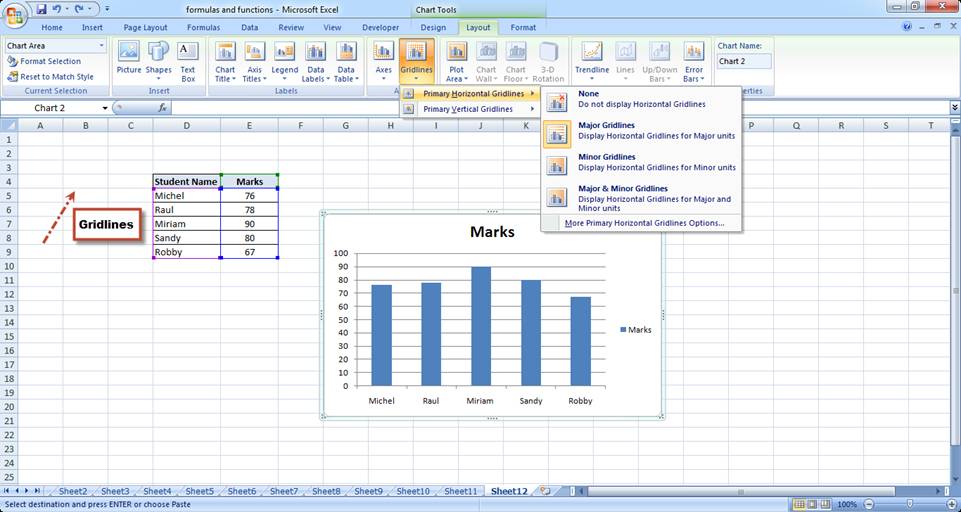
How to add data labels in excel graph. How To Create a Data Visualization in Excel (Plus Types) Give each column in your spreadsheet a title and arrange your data so each number is in a separate column. Different charts arrange titles in different areas, so you can run a test to see where your columns' titles appear on your visualization. You can also edit the titles of your charts later in the process. 2. Highlight your included data 12 Best Line Graph Maker Tools For Creating Stunning Line Graphs [2022 ... Introduction to Line Graph: There are eight types of line graphs, i.e. linear, power, quadratic, polynomial, rational, exponential, sinusoidal, and logarithmic. Line graph makers include the features of colors, fonts, and labels. The line graph makers will allow from 15 to 40 units on the X-axis and 15 to 50 units on the Y-axis for data. Figures (graphs and images) - APA 7th Referencing Style Guide - Library ... A figure may be a chart, a graph, a photograph, a drawing, or any other illustration or nontextual depiction. Any type of illustration or image other than a table is referred to as a figure. Figure Components. Number: The figure number (e.g., Figure 1) appears above the figure in bold. Title: The figure title appears one double-spaced line below the figure number in Italic Title Case. Two level axis in Excel chart not showing • AuditExcel.co.za You can easily do this by: Right clicking on the horizontal access and choosing Format Axis Choose the Axis options (little column chart symbol) Click on the Labels dropdown Change the 'Specify Interval Unit' to 1 If you want you can make it look neater by ticking the Multi Level Category Labels

how to edit a legend in Excel — storytelling with data How to do it in Excel: Click on your graph, and then in your Excel ribbon, select the "Format" tab next to the "Chart Design" tab. Towards the left hand side of your ribbon, click on the icon of a text box. That will place a blank text box in your Chart Area, which you can move, edit, and format just like a regular text box. How to make a graph or chart in Google Sheets - Spreadsheet Class To make a graph or a chart in Google Sheets, follow these steps: Click "Insert", on the top toolbar menu. Click "Chart", which opens the chart editor. Select the type of chart that you want, from the "Chart type" drop-down menu. Enter the data range that contains the data for your chart or graph. (Optional) Click the "Customize ... Understand charts: Underlying data and chart representation (model ... You can specify the data description XML string while you are creating a chart using the SavedQueryVisualization.DataDescription or UserQueryVisualization.DataDescription for the organization-owned or user-owned chart respectively. The data description XML string contains the following two elements: and . Note How To Show Two Sets of Data on One Graph in Excel To do so, click and drag your mouse across all the data you want, including the names of the columns and rows. You can check that you selected the data by looking for the cells to be gray instead of white. 3. Click the "Insert" tab and then look at the "Recommended Charts" in the charts group

Create and Modify a Chart Programmatically - DevExpress Refer to the following section for information on how to organize data in the source range to create a specific chart: Arrange Worksheet Data to Create a Chart. C#. VB.NET. // Create a column chart using a cell range as a data source. Chart chart = worksheet.Charts.Add (ChartType.ColumnClustered, worksheet ["B2:F6"]); Scatter, bubble, and dot plot charts in Power BI - Power BI Open the Analytics pane to add additional information to your visualization. Add a Median line. Select Median line > Add. By default, Power BI adds a median line for Sales per sq ft. This isn't very helpful since we can see that there are 10 data points and know that the median will be created with five data points on each side. How do you label data points in Excel? - profitclaims.com Right click the data series in the chart, and select Add Data Labels > Add Data Labels from the context menu to add data labels. 2. Click any data label to select all data labels, and then click the specified data label to select it only in the chart. 3. How to Add a Secondary Axis to Charts in Microsoft Excel? Adding a Secondary Axis in Excel - Step-by-Step Guide 1. Download the sample US quarterly GDP data here. …. 2. Open the file in Excel, and get the quarterly GDP growth by dividing the first difference of quarterly GDP with the previous quarter's GDP. 3. Select the GDP column (second column) and create a line chart.

Excel Dot Plots and other charts to display students data

How to add an Excel second y-axis (plus benefits and tips) Add data to a spreadsheet To create a graph in Excel, open a blank spreadsheet and add some data to the first three rows. You may see that the first row correlates with the x-axis and the second row with the y-axis. In this instance, the third row can be the secondary or second y-axis. 2. Make a chart using the data

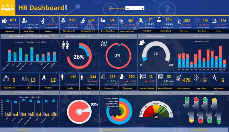
Excel Advanced Dashboard

Types of Graphs - Top 10 Graphs for Your Data You Must Use Add data labels #8 Gauge Chart The gauge chart is perfect for graphing a single data point and showing where that result fits on a scale from "bad" to "good." Gauges are an advanced type of graph, as Excel doesn't have a standard template for making them. To build one you have to combine a pie and a doughnut.

Excel rotate radar chart - Stack Overflow

How to add a single vertical bar to a Microsoft Excel line chart Click anywhere inside the data set, which is a Table object named Sales in this case. Click the Insert tab. In the Charts group, click Insert Line or Area Chart and choose Line with Markers (...

How to make Excel chart with two y axis, with bar and line chart, dual axis column chart, axis ...

A Beginner's Guide on How to Plot a Graph in Excel Firstly, select the cells that have the data you want to use in your graph by clicking and dragging across the cells. Secondly, once the text is highlighted, you can select a graph. Click the Insert tab and click your chart or graph you wish to use. Now you have your graph. Finally, customize your graph for aesthetics and convenience.

How to Add Data Labels to your Excel Chart in Excel 2013 - YouTube

Excel Line Column Chart With 2 Axes - Contextures Excel Tips Select any cell in the data range. On the Excel Ribbon, click Insert tab, then click Column Chart. In the 2-D Column section, click the first chart type -- 2D Clustered Column chart. This creates a chart that is embedded on the active worksheet, with both the series shown as columns. Product names are shown in the axis labels on the horizontal ...

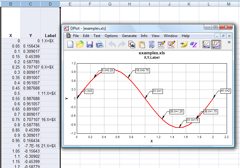
DPlot Windows software for Excel users to create presentation quality graphs

How to Use Drop Down Menus to Make Interactive Charts and Dashboards in ... Okay, so now the data will be automatically updated each time someone chooses one of the outlets in the drop down we created. Time to create an interactive chart. Go to 'Insert Menu', open 'Charts', and select 'Line with Markers'. This chart should appear: You can later customize the color and other elements of the chart in any way you like.

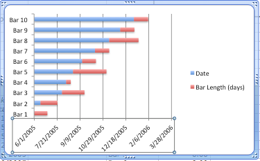
Excel Timelines

How to Create a Dynamic Chart Title in Excel Steps to Create Dynamic Chart Title in Excel Converting a normal chart title into a dynamic one is simple. But before that, you need a cell which you can link with the title. Here are the steps: Select chart title in your chart. Go to the formula bar and type =. Select the cell which you want to link with chart title. Hit enter.

Basic Excel Chart Formatting - MS Excel Charting Tutorial Part 4 | Vertical Horizons

14 Best Types of Charts and Graphs for Data Visualization - HubSpot Download the Excel templates mentioned in the video here. ... Use horizontal labels to improve readability. Start the y-axis at 0 to appropriately reflect the values in your graph. 2. Column Chart ... They make it simple to add a lot of data on a single chart or to make a point with limited space.

Share :